Hemispherical Infrared - Software
Software documentation for hemispherical infrared camera. From angle picking to combined image
Overview of the software
In this section will be covered the software aspects of this project. There will be a lot of stitching, camera parameters estimation as well as communication with the sensor and the servos. I hope this software can be useful to you, as such it is released under an Apache 2.0 License. Feel free to reach out if any part here is confusing or just to share ideas.
Software repositories are available here:
The softare is divided in a few components:
- A angle calculation “library” (in python) that is meant to go from the camera viewpoints to cubemaps and vice versa.
- A set of preparation tools (in python) that allow to select the capturing angles for the hemispherical camera
- A program to drive the servos and the sensors (in C++). This program stores the data in a TIFF file with custom metadata
- A set of programs to analyze the sensor data and project the thermal information onto cubemaps
- A program to estimate the sensor geometrical information from calibration measurements
- A program to display the cubemap in a browser using Three.JS
- And some extra notes on quaternions and raspberry pi set-up
Angles calculation “library”
This library does the heavy lifting between camera and cubemap information, it does the rotation/overlap/homography/interpolation/homogeneity calculations.
The small program demo_display_compute_steps.py illustrate several of the concepts below.
Here we will review the key files and functions of this library as well as some results illustration.
transf_mat.py
This file contains helper functions for quaternions, rotation matrices and homographies. This is typically time consuming to write but easy to use.
The way the transfer is done is that we sample the cubemap views at a certain resolution and for each cubemap view point and for each sensor we compute if there is a corresponding sensor pixel in this cubemap pixel, if yes what is the coordinate. In other words we search the sensors from the cubemap and not the opposite.
We can follow this code from the high level functions to lower level ones
compute_all_matrices - mostly helper function
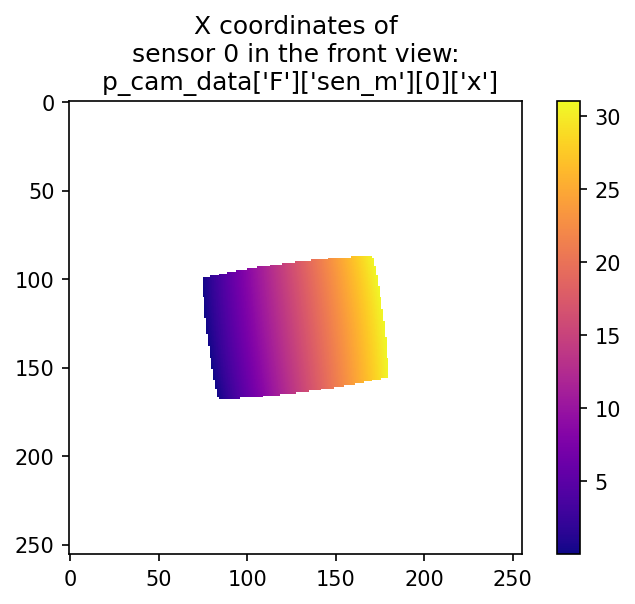
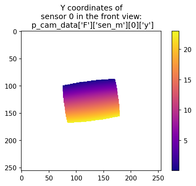
This function takes the sensor data and the cubemap data, and prepare a few matrices for each cubemap: sen_m and sen_nm.
These matrices contain what sensor is visible at which pixel of the cubemap AND the respective (“float”) X and Y coordinates on the sensor image.
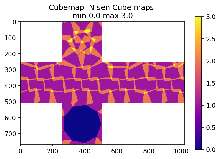
Then reconstructing the image consists in obtaining the sensor data, and managing the overlapping and interpolation. This function is an helper function that calls compute_pixel_mat for each sensor for each cubemap. Then merge the data and accumulate the number of sensors visible for each pixel of the map.
Taken on several sensors views this is the kind of results that are obtained for the number of overlapping pixels
compute_pixel_mat - key function
This function computes for a given view of the cubemap and a given sensor position the coordinates of the pixels of the sensor for each pixel of the view.
This function does the following
- compute the transfer homography matrix between the sensor view and the cubemap view using
compute_transfer_mat. This is where the orientation and field of views of both cameras are taken into account. - this matrix is applied to the coordinates of the cubemap, using an homography transformation. This tells for each point of the cubemap, for this view of the sensor, what is the image coordinate in the sensor view frame of reference.
- The distortion of the camera is taken into account computing the “inverse distortion” on the coordinates. Ie where in the sensor this theoretical angle (aka X, Y coordinates on the sensor image) is to be found knowing that the sensor have a certain distortion.
- So far the computed coordinates can be outside of the sensor view, for example we can have absolute values > 1 from the previous calculations
- We covert the normalized sensor pixel coordinates into “real pixel coordinates”
Note: The results are floating point values, interpolation is done elsewhere when information is merged.
For the case of one sensor view on the front cubemap, we obtain the lookup information to get the sensor pixel data:
compute_cubemap - key function
This function takes sensor data, pre computed coordinate matrices (from compute_all_matrices/compute_pixel_mat) and compute the cubemap view of the thermal information.
This function does
- the pixel interpolation
- sensor overlap management. When several sensors have view on a certain points of the cubemap the resulting information will be weighted versus the distance to the center of each sensor view (the closer to the center the more weight), this allow for a smoother transition.
- Sensor homogeneity compensation, currently a model in cos(theta)^4 (where theta is the angle compared to the sensor view principal axis) is used. It is a “simple” vignetting model, for which the parameters are adjusted by hand
NOTE: This is in this function that advanced computation can be done like super resolution and automatic sensor homogeneity correction
This is an example result
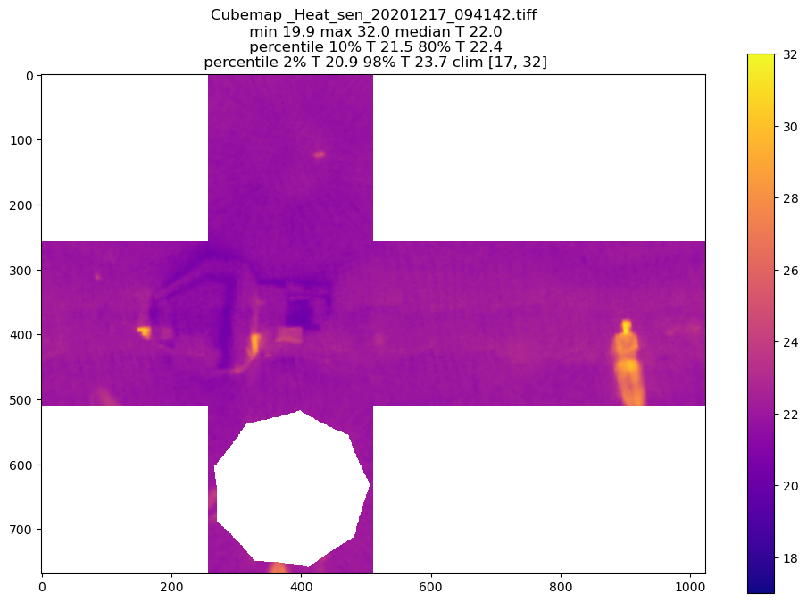
This is WITHOUT vignetting correction

compute_transfer_mat - key function
This function computes the transfer matrix between two cameras, for example between a viewpoint camera (eg. FRONT) and the camera of the sensor at a specific angle. This matrix is then used to compute the mapping from pixels to pixels.
Example result for a front view and a front viewing sensor (gamma_i is the rotation about the sensor axis)
Cubemap data (destination camera)     {'alpha': 0, 'beta': 0, 'HFOV': 90, 'VFOV': 90, 'HNPIX': 256, 'VNPIX': 256}
Sensor data  (source camera)          {'alpha': 0, 'beta_i': 0, 'HFOV': 45.64884636, 'VFOV': 33.6037171, 'gamma_i': 7.36132776, 'distortion': -2.87108226, 'HNPIX': 32, 'VNPIX': 24}

Camera matrix of the source camera
	 2.4  0.0  0.0
	 0.0  3.3  0.0
	 0.0  0.0  1.0
Rotation matrix of the source camera
	 1.0 -0.1  0.0
	 0.1  1.0  0.0
	 0.0  0.0  1.0
Inverse of the Rotation matrix of the destination camera
	 1.0  0.0  0.0
	 0.0  1.0  0.0
	 0.0  0.0  1.0
Inverse of the Camera matrix of the destination camera
	 1.0  0.0  0.0
	 0.0  1.0  0.0
	 0.0  0.0  1.0
Final transfer matrix
	 2.4 -0.3  0.0
	 0.4  3.3  0.0
	 0.0  0.0  1.0
gen_cubemap_data - helper function
This is an helper function that generate the camera data for the cubemaps given a number of pixels
Example result:
{'F': {'alpha': 0, 'beta': 0, 'HFOV': 90, 'VFOV': 90, 'HNPIX': 256, 'VNPIX': 256},
    'L': {'alpha': 90, 'beta': 0, 'HFOV': 90, 'VFOV': 90, 'HNPIX': 256, 'VNPIX': 256},
    'R': {'alpha': 270, 'beta': 0, 'HFOV': 90, 'VFOV': 90, 'HNPIX': 256, 'VNPIX': 256},
    'B': {'alpha': 180, 'beta': 0, 'HFOV': 90, 'VFOV': 90, 'HNPIX': 256, 'VNPIX': 256},
    'T': {'alpha': 0, 'beta': 90, 'HFOV': 90, 'VFOV': 90, 'HNPIX': 256, 'VNPIX': 256},
    'Bo': {'alpha': 0, 'beta': -90, 'HFOV': 90, 'VFOV': 90, 'HNPIX': 256, 'VNPIX': 256}}
plotting.py
Helper functions to display cubemap data
Preparation/angle optimization tools
robot_optimize_angles.py
Preparation file to select the angles on which the robot will run. It is mostly manual as this is typically run once, but allow to see what is the predicted sensor overlap. It is a good file to get familiar with the way the code runs. Some aspects of it are a bit clunky as the code versus configuration should be more separated…. It also compute the angular displacement of the servo between each step. The spirit is the angle list will be first built in a naive way, per “layer”, then arranged to minimize servo displacement. This arrangement step could be done automatically but the current needs for automation were to low to justify the efforts.
The goal of this file is to obtain an overlap map to make sure the images are taken in a correct way. This computation is based on the angle library so sensor parameters are taken into account. Here spherical aberration, Horizontal and Vertical Field of view and rotation about its axis. The latter is why the sub images appear tilted in the image below.
This is what a typical result can look like, with 37 images and a 55FOV sensors. This plot shows for each point of the cubemap how many independent images will be taken given a certain list of angle pairs for the servo positions. In that case we have a good coverage, and reasonable overlap.
This is the heat map for the calibration list, The center is horizontally at 45 degrees to take into account the prototype mounting.
It also print the list of angles in a readable format for the servo driving program
Here is your arranged list by hand !!! , you have 37 positions
Sensor   0	 Alpha   201.0	 Beta_i   -32.0 	 DAlpha    201.0	 DBeta_i   -32.0
Sensor   1	 Alpha   241.0	 Beta_i   -32.0 	 DAlpha     40.0	 DBeta_i     0.0
Sensor   2	 Alpha   281.0	 Beta_i   -32.0 	 DAlpha     40.0	 DBeta_i     0.0
Sensor   3	 Alpha   321.0	 Beta_i   -32.0 	 DAlpha     40.0	 DBeta_i     0.0
Sensor   4	 Alpha   361.0	 Beta_i   -32.0 	 DAlpha     40.0	 DBeta_i     0.0
Sensor   5	 Alpha    41.0	 Beta_i   -32.0 	 DAlpha   -320.0	 DBeta_i     0.0
Sensor   6	 Alpha    81.0	 Beta_i   -32.0 	 DAlpha     40.0	 DBeta_i     0.0
Sensor   7	 Alpha   121.0	 Beta_i   -32.0 	 DAlpha     40.0	 DBeta_i     0.0
Sensor   8	 Alpha   161.0	 Beta_i   -32.0 	 DAlpha     40.0	 DBeta_i     0.0
Sensor  17	 Alpha   141.0	 Beta_i    -4.0 	 DAlpha    -20.0	 DBeta_i    28.0
Sensor  16	 Alpha   101.0	 Beta_i    -4.0 	 DAlpha    -40.0	 DBeta_i     0.0
.......
# ==== Angles for angles.txt =========
201.00  -32.00
241.00  -32.00
281.00  -32.00
321.00  -32.00
361.00  -32.00
 41.00  -32.00
 81.00  -32.00
121.00  -32.00
161.00  -32.00
.......
Motion and capture software
The software is C/C++ code, it expect the Robotis SDK to be properly installed, a modified version of the Melexis library is shipped with the code.
I use ID 20 for the bottom servo, ID 21 for the top servo. They are left at the default speed of 1Mb/s. If you want to change servo specific parameters, see examples/DXL_info.h and examples/DXL_info.h
The code is in the infrared-capture repository and does the interface with the robotis and melexis librairies.
It does the motion control, check motion convergence, clear sensor data, capture infrared image, store it and move again.
The default folder for image storage is ../data/images_servo and the main program is Servo_360_DXL
The code would need some clean up for more “configurability” but is pretty much self explanatory.
It also includes a small piece of code to change the i2c address of the infrared sensor if necessary (please read the code and the datasheet before using it !)
Sensor calibration software
The concept
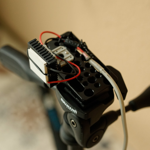
The idea is to image a point source under a set of angles, then knowing the angles at which we imaged it (thanks to the servos) we can fit the camera parameters.
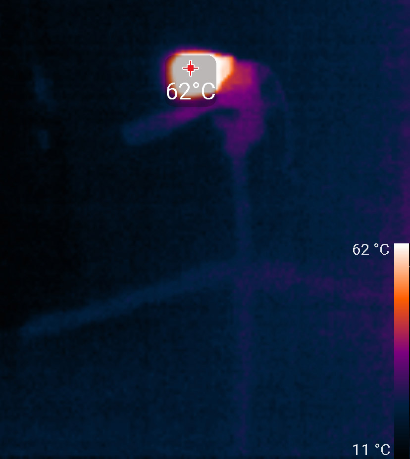
Below you can find an image of the thermal source I used (a thermoelectric element plugged on a phone charger) in visible and with a Seek infrared camera.
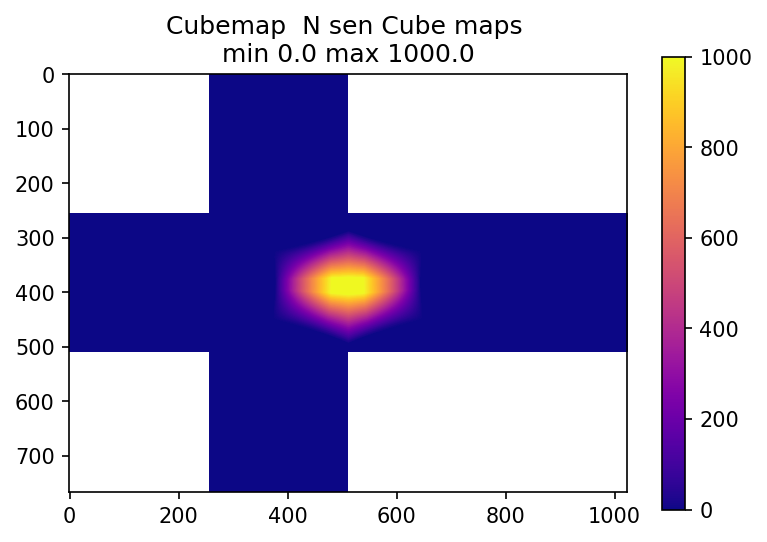
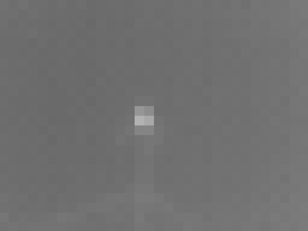
This is the same source viewed by the melexis sensor
The parameters we adjust are the following:
| Parameter | Description |
|---|---|
| par_dh | Horizontal “center” this one is due to the alignment between the camera and the source and can be ignored |
| par_dv | Vertical “center” this one is due to the alignment between the camera and the source and can be ignored |
| par_dz | Rotation about the sensor axis. This one is due to how the sensor is mounted and soldered. Without a specifically made holder it can be quite high. |
| par_HFOV | Camera horizontal field of view |
| par_VFOV | Camera vertical field of view |
| d_a1 | Camera spherical aberration |
camera_calibration.py
This file contains the camera calibration program. It uses curve_fit from the scipy.optimize package.
The center estimation (sensors_find_maxima) is assuming it’s a gaussian hot spot to perform sub pixel estimation and use the <x.P(X)> value where X is the pixel position and P(X) is the normalized itensity
It also implement the distance function and the associated calculations in guess_images_centers_quat
results
The distance reported in these results is the average distance between the maximum centers and their expected position in pixels. Without any fit beside the centers, the average distance is 1.4px, after fit it is 0.17px
The fit results are:
| Parameter | Fit | Expected value | Description |
|---|---|---|---|
| par_dz | 7.45 | 0 | Rotation about the sensor axis. This one is due to how the sensor is mounted and soldered. Without a specifically made holder it can be quite high. |
| par_HFOV | 46.1 | 55 | Camera horizontal field of view |
| par_VFOV | 33.8 | 35 | Camera vertical field of view |
| d_a1 | -2.33 | 0 | Camera spherical aberration |
One can notice that the horizontal field of view is pretty different from expected, and the pixels are not square. The spherical distortion is non negligible for stitching purposes. The remaining distance is well in the subpixel range and can be due to either the difficulty to estimate the center of the source or the mechanical imprecision
For the camera distortion, this is the function used
def camera_distortion(x,y,a1):
    r2 = x**2+y**2
    a1 /= 10000
    xd = (1 + a1*r2)*x
    yd = (1 + a1*r2)*y
    return xd,yd
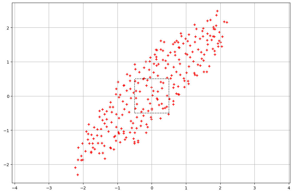
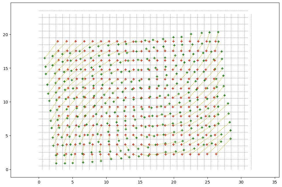
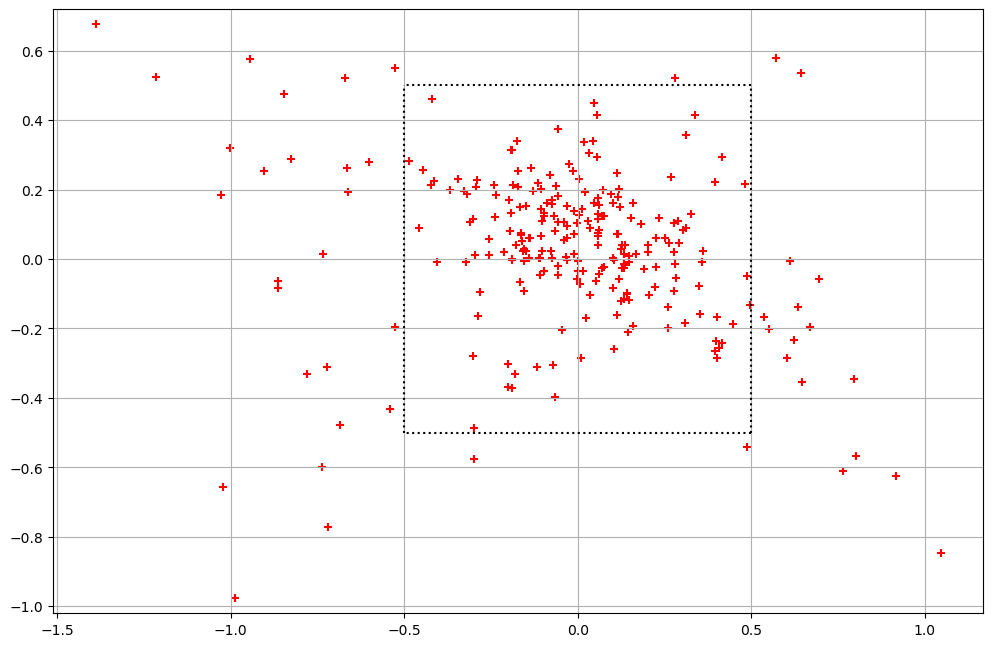
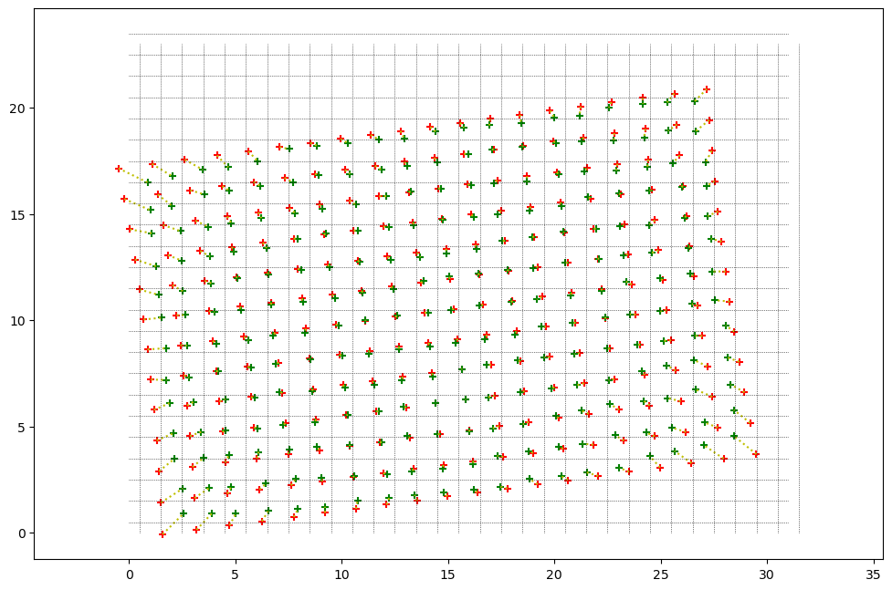
Below you can find a few illustrations of the results, the scatter plot corresponds to the XY distance for each measurement between expected and estimated. The cross plot is an illustration of the same in the image plane.
Dz = 0; HFOV = 55; VFOV = 35; a1 = 0 : No calibration
Dz = 7.52; HFOV = 55; VFOV = 35; a1 = 0 : Sensor rotation calibrated
Dz = 7.52; HFOV = 46.1; VFOV = 33.7; a1 = 0 : Sensor rotation, Field of View calibrated
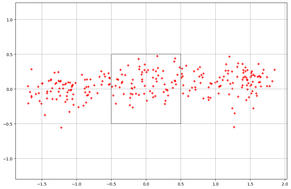
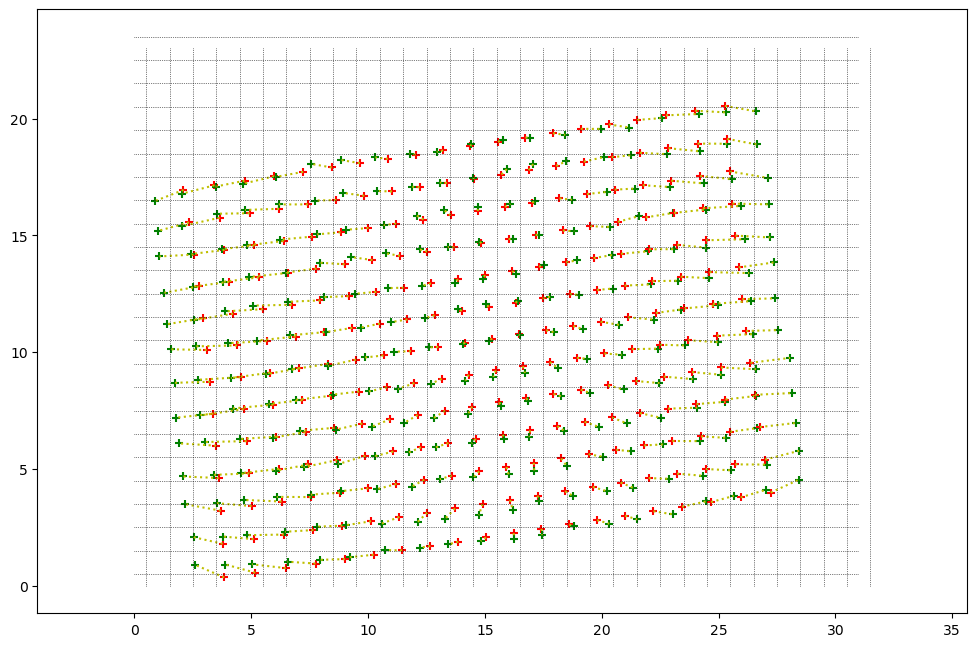
Final fit results
Dz = 7.45; HFOV = 46.1; VFOV = 33.8; a1 = -2.33 : Everything (Sensor rotation, Field of View, distortion) calibrated
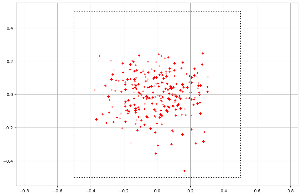
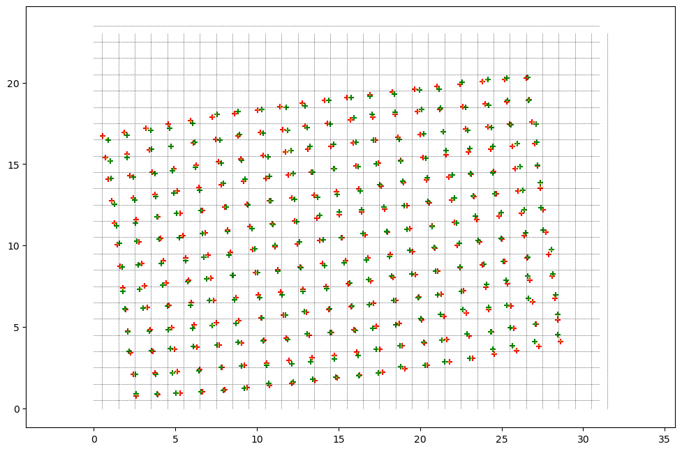
One can see the pretty impressive difference and the value of this calibration work !
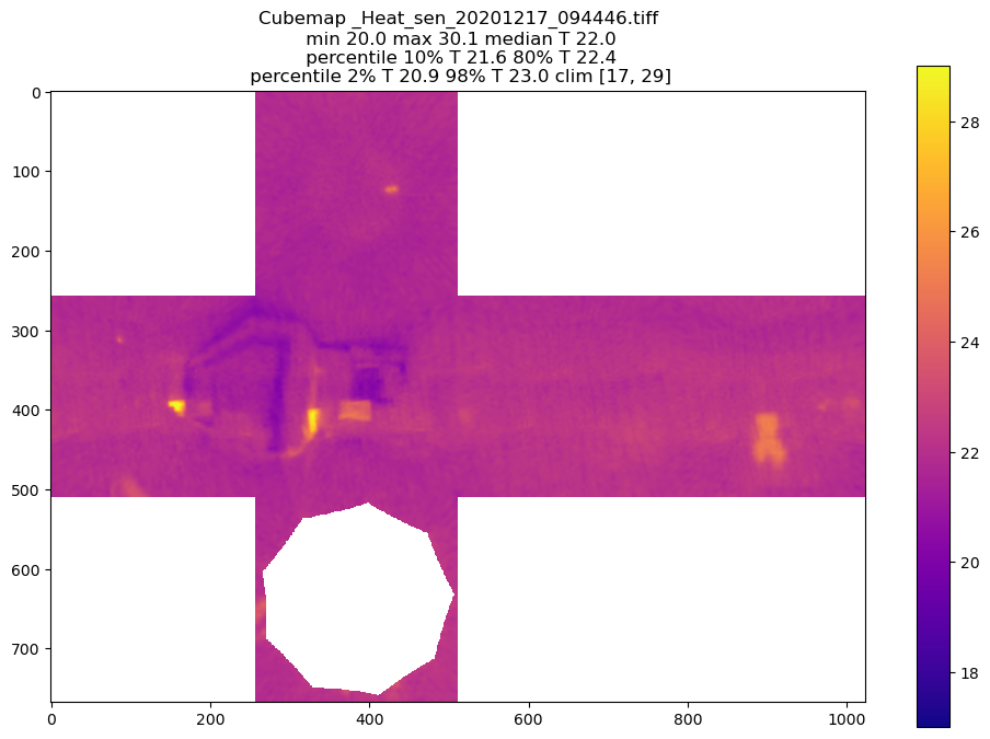
Image analysis software
file_loader.py - Load a single tiff file
This file loads the tiff and parse the metadata to fill the sensor information
file_to_cube.py - Load a tiff file and convert into cubemap
This file is the one you have to look at to load and convert measurement data.
It will load the tiff file, generate the cubemap camera information, then ask the main library to do the cubemap from the pixel data.
It can display the cubemap in several formats including texture files for 3D visualization
Just for the fun, once I left the room we can see the residual heat on the couch
Display the cubemap using three JS
Once a cubemap is obtained it can be displayed in a more interesting way like below
Or we can display cubemap videos easily with three JS
A few notes on quaternions
In the software I am using quaternions to describe rotations. Once the set-up is in place, these are a very practical tool to handle arbitrary rotations. The image stitching is the rotation of the two servos and the rotation associated to the sensor pixels versus the rotation of the point of the cubemap. So a robust rotation parametrization is key. In this project I have decided to use quaternions, as they do not suffer from gimbal lock, rotation combinations are easy (it’s a kind of product), and they are simple to invert. They are not easy to parametrize directly but the conversion to other rotation parametrizations is well documented.
Quaternions are described in various places, here you can find a link on the key equations used and it should help for notation
TIFF storage and metadata
In order to store the angles and the imaging conditions, we add metadata to the TIFF file containing the raw measurements. The two following sections describe the metadata syntax as well as where is the metadata stored in the TIFF file.
The metadata is stored in the tag 270: ImageDescription.
This is one example of metadata
THDS_V0.04//NIM:37//ANH:201.00;241.00;281.00;321.00;361.00;41.00;81.00;121.00;161.00;141.00;101.00;61.00;21.00;341.00;301.00;261.00;221.00;181.00;201.00;241.00;281.00;321.00;361.00;41.00;81.00;121.00;161.00;129.57;78.14;26.71;335.29;283.86;232.43;181.00;181.00;301.00;61.00//ANV:-32.00;-32.00;-32.00;-32.00;-32.00;-32.00;-32.00;-32.00;-32.00;-4.00;-4.00;-4.00;-4.00;-4.00;-4.00;-4.00;-4.00;-4.00;23.00;23.00;23.00;23.00;23.00;23.00;23.00;23.00;23.00;51.00;51.00;51.00;51.00;51.00;51.00;51.00;76.00;76.00;76.00//TA_S:27.47;27.48;27.47;27.47;27.47;27.45;27.45;27.45;27.44;27.44;27.43;27.44;27.44;27.44;27.43;27.43;27.43;27.43;27.44;27.43;27.44;27.42;27.42;27.41;27.31;27.31;27.30;27.31;27.31;27.31;27.31;27.30;27.29;27.39;27.26;27.28;27.26//SFPS:1//TI_SD:20201211//TI_ST:091058//TI_DU:150.15
Metadata definition
The tags start with an header, here THDS_V0.04 followed by pairs Name:Value. Each field is separated by \\
This is the descriptions of the field
| Field Name | Value Description |
|---|---|
| NIM | (always first) the number of images in the file. Example NIM:3 |
| ANH | The angles in the “Horizontal plane”, corresponding to Y in the angle convention. Each angle is separated by a semicolon ; and in a preffered format %.2f. Example ANH:201.00;241.00;281.00 |
| ANV | The angles in the “Vertical plane”, corresponding to Xi in the angle convention. Each angle is separated by a semicolon ; and in a preffered format %.2f. Example ANV:-32.00;-32.00;-32.00 |
| SFPS | The sensor integration time in seconds. Example SFPS:1 |
| TA_S | The sensor internal temperature for each image in Degree Celcius. Example TA_S:27.47;27.48;27.47 |
| TI_SD | The measurement start date, format %Y%m%d. Example TI_SD:20201211 |
| TI_ST | The measurement start time, format %H%M%S. Example TI_ST:091058 |
| TI_DU | The measurement duration. Example TI_DU:150.15 |
| SEN | (Future use) The sensor model. Example SEN:MLX90640_110 |
| TI_IO | (Future use) The time from start for each image. Example TI_IO:0;2.3;5.8 |
| TEMP | (Future use) The overall temperature. Example TEMP:21.5 |
Metadata storage
This is the structure of the generated TIFF file. The code is inspired from (Paul Bourke http://paulbourke.net/ work). These are the sections of the generated TIFF file in order. Tiff files can be complex, below is the simplest TIFF file that suited the needs of the project.
| Field Name | Value | Description |
|---|---|---|
| HEADER | 0x4d4d002a | Big endian & TIFF identifier. Size: 4bytes |
| FIRST IFD OFFSET | “Nx * Ny * 2 + 8” | Where to find the “Image File Directory” which is the description of the file information. Size: 4bytes |
| IMAGE_DATA | Image data | Rraw grayscale, 2Bytes per pixel. Size: Nx * Ny * 2 Bytes |
| This is the start of the IFD | ||
| TAG N | 12 | The number of tags in the IFD. Size 2Bytes |
| TAG 0x00fe: Image type | 0 | |
| TAG 0x0100: Image Width | Nx | Number of horizontal pixels |
| TAG 0x0101: Image Height | Ny | Number of vertical pixels |
| TAG 0x0102: Bits/sample | 16 | Grayscale 2bytes/pixel |
| TAG 0x0103: Compression | 1 | uncompressed |
| TAG 0x0106: Photometric Interpretation | 1 | Minimum is black |
| TAG 0x0111: Strip Offsets | 8 | This is the pointer in bytes on where to find the data. As the data is at the beginning after the two headers its value is 4 + 4 = 8bytes |
| TAG 0x0112: Orientation | 1 | First pixel is top left |
| TAG 0x0115: SamplesPerPixel | 1 | Grayscale image = 1 sample per pixel |
| TAG 0x0117: StripByteCounts | Nx * Ny * 2 | Number of bytes in the strip. We are doing a single strip image so that’s the size of the image data |
| TAG 0x011C: PlanarConfiguration | 1 | How the components of each pixel are stored. 1 = The component values for each pixel are stored contiguously |
| TAG 0x010E: ImageDescription | Pointer to data | TAG_N (tag data len): Even String length. tag data Offset: 8 (Image header) + Nx * Ny * 2 ( Image data ) + 2 (Tag number field size) + 12*12 (Tag information, each tag is 12 Bytes total) + 4 (Next IFD offset field) |
| NEXT IFD OFFSET | 0x00000000 | The image is over so we do not have another IFD |
| IMAGE_DESCRIPTION | our metadata | See appropriate section |
| EOF | ‘neo’ | Normal tiff parsers must not reach here because the image is over, but for the fun I added a footer. |
Reading metadata in python
As simple as this
from PIL import Image
img = Image.open('xxx.tiff')
metadata = img.tag_v2.get(270,"").replace("\x00","")
Raspberry pi set-up
run raspi_config and set-up
- ssh (if you use it)
- enable i2c port
- serial port (if using lidar): no console and hardware enabled
edit /boot/config.txt and adjust the i2c_frequency (200kHz worked fine for me) and if using lidar, disable bluetooth to free the serial port by adding dtoverlay=pi3-disable-bt-overlay
if using lidar on serial, I run also this command to disable the bluetooth sudo systemctl disable hciuart
Note: for remote display with rdp sudo apt purge realvnc-vnc-server && sudo apt install xrdp. Client wise it works on linux/windows and iPad but not all apps (iteleport works fine)
Raspberry pi client and AP simultaneously
As this is meant to be a portable device, having an AP mode on the PI can be useful. Fortunately the controller can do both like in this tutorial.
The key point that is different from the tutorial is the fact that both interfaces have to be up in a certain order and I use /etc/network/interfaces to do that, and I also have set up two potential wifi to connect to (house and phone)
source-directory /etc/network/interfaces.d

auto lo
auto ap0
auto wlan0
iface lo inet loopback

allow-hotplug ap0
iface ap0 inet static
    address 192.168.10.1
    netmask 255.255.255.0
    hostapd /etc/hostapd/hostapd.conf

allow-hotplug wlan0
iface wlan0 inet manual
    pre-up ifup ap0
    wpa-roam /etc/wpa_supplicant/wpa_supplicant.conf
    post-down ifdown ap0
iface AP1 inet dhcp
iface AP2 inet dhcp
Get your mac with iw dev and set up /etc/udev/rules.d/70-persistent-net.rules
SUBSYSTEM=="ieee80211", ACTION=="add|change", ATTR{macaddress}=="b8:27:eb:dc:ec:7c", KERNEL=="phy0", RUN+="/sbin/iw phy phy0 interface add ap0 type __ap", RUN+="/bin/ip link set ap0 address b8:27:eb:dc:ec:7c
I followed the tutorial for /etc/dnsmasq.conf, /etc/default/hostapd,/etc/hostapd/hostapd.conf. Concerning the /etc/wpa_supplicant/wpa_supplicant.conf I set it up this way.
country=US
ctrl_interface=DIR=/var/run/wpa_supplicant GROUP=netdev
update_config=1

network={
    ssid="SSID_1"
    psk="PAAASSSSSS1"
    id_str="AP1"
}
network={
    ssid="SSID_2"
    psk="PAAASSSSSS2"
    id_str="AP2"
}
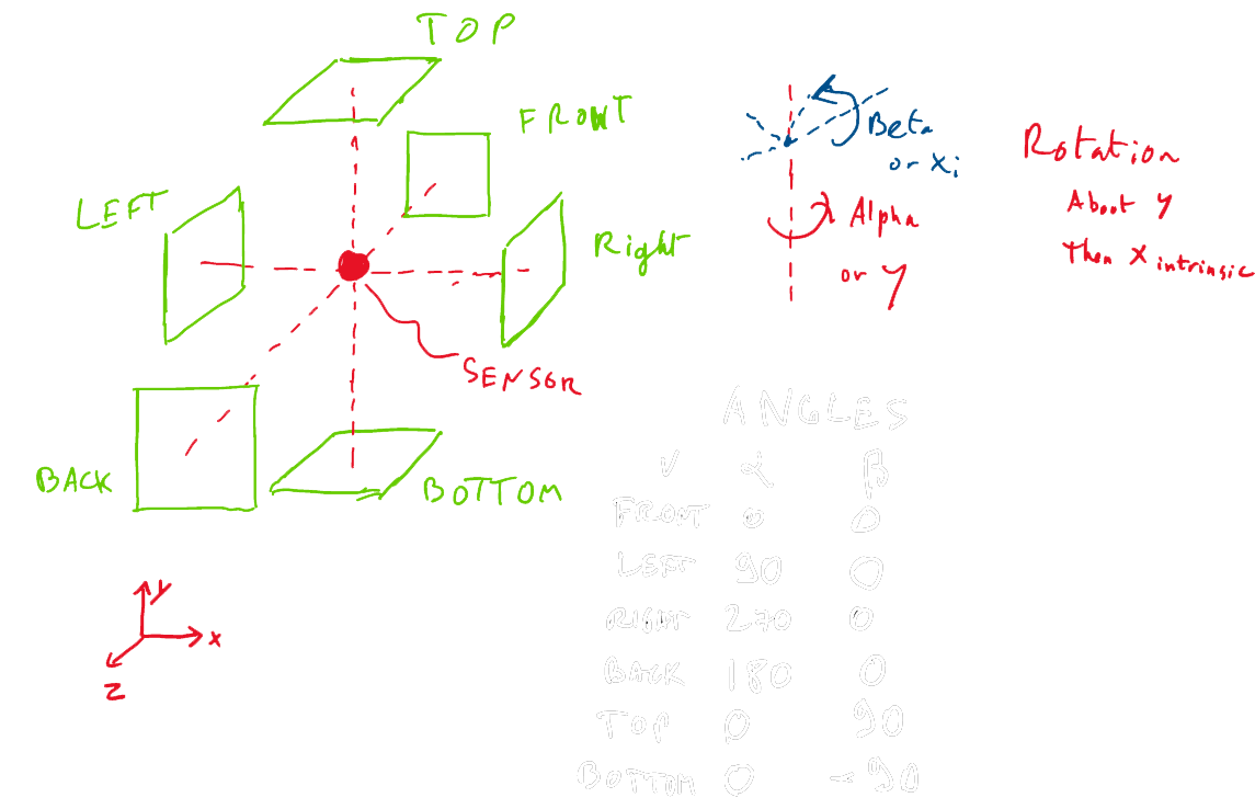
Angles convention
Here are the conventions used for the angles in this project
Project maintained by Brice Dubost-Vedrenne Theme jekyll-theme-midnight by mattgraham modified by Brice Dubost-Vedrenne

This work is licensed under a Creative Commons Attribution-NonCommercial-ShareAlike 4.0 International License.